2.3. Curve transformation
2.3.1. Transform airfoil
Figure 2.3.1 shows the transformation of an airfoil. It takes three steps in order: translation (dx, dy), scale (scale, x0, y0), and rotation (rot, xr, yr, projection).
 1xu_, xl_, yu_, yl_ = transform(x0, x0, yu0, yl0, rot=20, projection=True)           # black
 2
 3xu_, xl_, yu_, yl_ = transform(x0, x0, yu0, yl0, scale=1.5, rot=20,
 4    dx=xLE-0.0, dy=yLE-0.0, x0=None, y0=None, xr=None, yr=None, projection=False)   # blue
 5
 6xu_, xl_, yu_, yl_ = transform(x0, x0, yu0, yl0, scale=1.5, rot=-10,
 7    dx=xTE-1.0, dy=yTE-0.0, x0=xTE, y0=yTE, xr=xTE, yr=yTE, projection=False)       # green
 8
 9xu_, xl_, yu_, yl_ = transform(x0, x0, yu0, yl0, scale=1.5, rot=-10,
10    dx=0.0, dy=0.0, x0=0.5, y0=0.0, xr=None, yr=None, projection=False)             # red
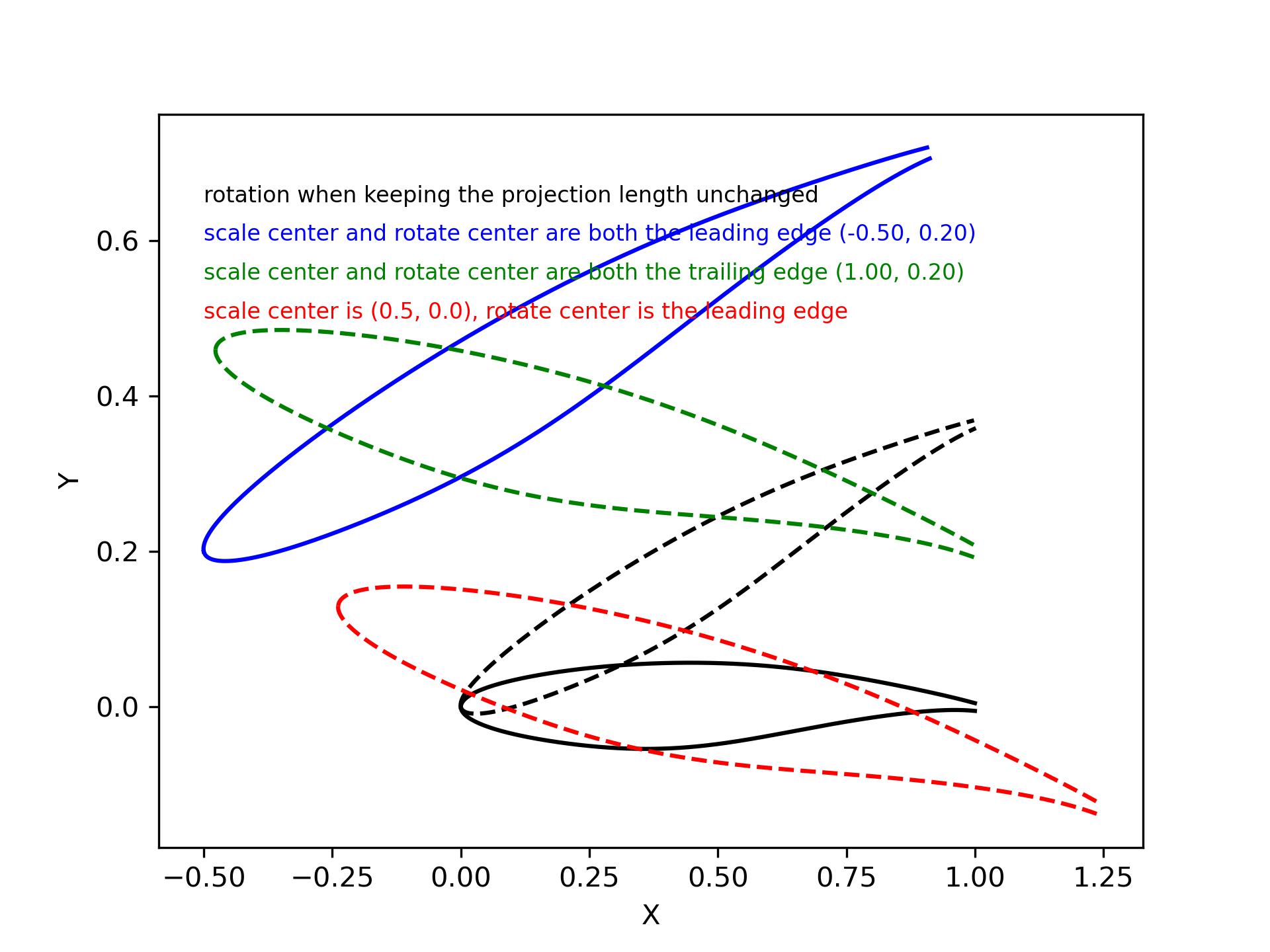
Figure 2.3.1 Transform airfoil
There are also a function rotate that can rotate a curve about the X, Y or Z axis. And a function rotate_vector that can rotate points about any given axis.
1x_, y_, z_ = rotate(x, y, z, angle=10, origin=[0, 0, 0], axis='Z')
2
3curve = rotate_vector(x, y, z, angle=10, origin=[0, 0, 0], axis_vector=[0,0,1])
2.3.2. Normalize airfoil
Figure 2.3.2 shows the normalization of any airfoil.
1xu_, yu_, xl_, yl_, twist, chord, tail = normalize_foil(xu, yu, xl, yl)
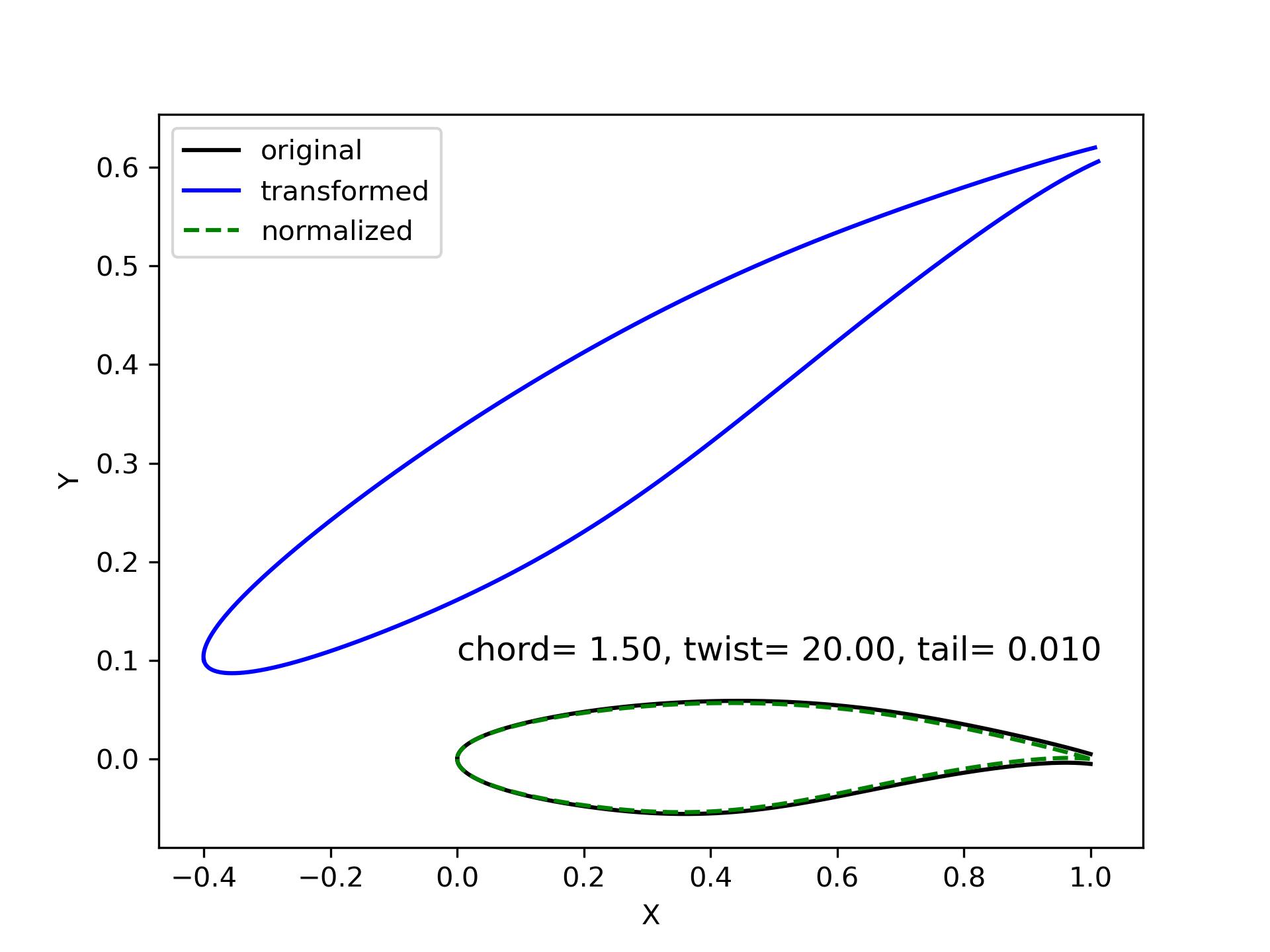
Figure 2.3.2 Normalize airfoil
2.3.3. Stretch curve
Figure 2.3.3 shows the result of stretching a curve. It linearly stretch a curve when a certain point (xf, yf) is fixed. The fixed point is suggested on one of the ends of the given curve. Otherwise, it may gives counterintuitive results, e.g., the green and red curves.
1xu_, yu_ = stretch_fixed_point(x0, yu0, dx=dx, dy=dy, xm=xm, ym=ym, xf=xf, yf=yf)

Figure 2.3.3 Stretch curve
2.3.4. Cylinder to plane
When we have a model of compressor, fan or turbine, the control sections of the blade are usually defined on cylinders. The section curve can be sliced by a cylinder (radius is \(r_0\)), the Cartesian coordinates are \(x, y, z\). We can transfer them to cylindrical coordinates \(r, \theta, z\). The transformation between cylindrical coordinates and Cartesian coordinates is Eq.2.3.1.
Then, we want to obtain the 2D curve on a X-Y plane, the coordinates are \(X, Y, Z\). The transformation is defined by Eq.2.3.2. This shows that the 2D curve is on plane \(Z=r_0\).
Figure 2.3.4 shows the cylinder curve and the corresponding plane curve.
An increment of the azimuth angle \(\theta\) leads to an increment of \(X\) (airfoil).
An increment of the \(z\) coordinate (blade) leads to the same displacement of \(Y\) (airfoil).
The radius of cylinder \(r_0\) is the \(Z\) coordinates of the plane (airfoil).
1x, y, z = toCylinder(X, Y, Z, flip=False, origin=[0, 0])
2
3X, Y, Z = fromCylinder(x, y, z, flip=False, origin=[0, 0])
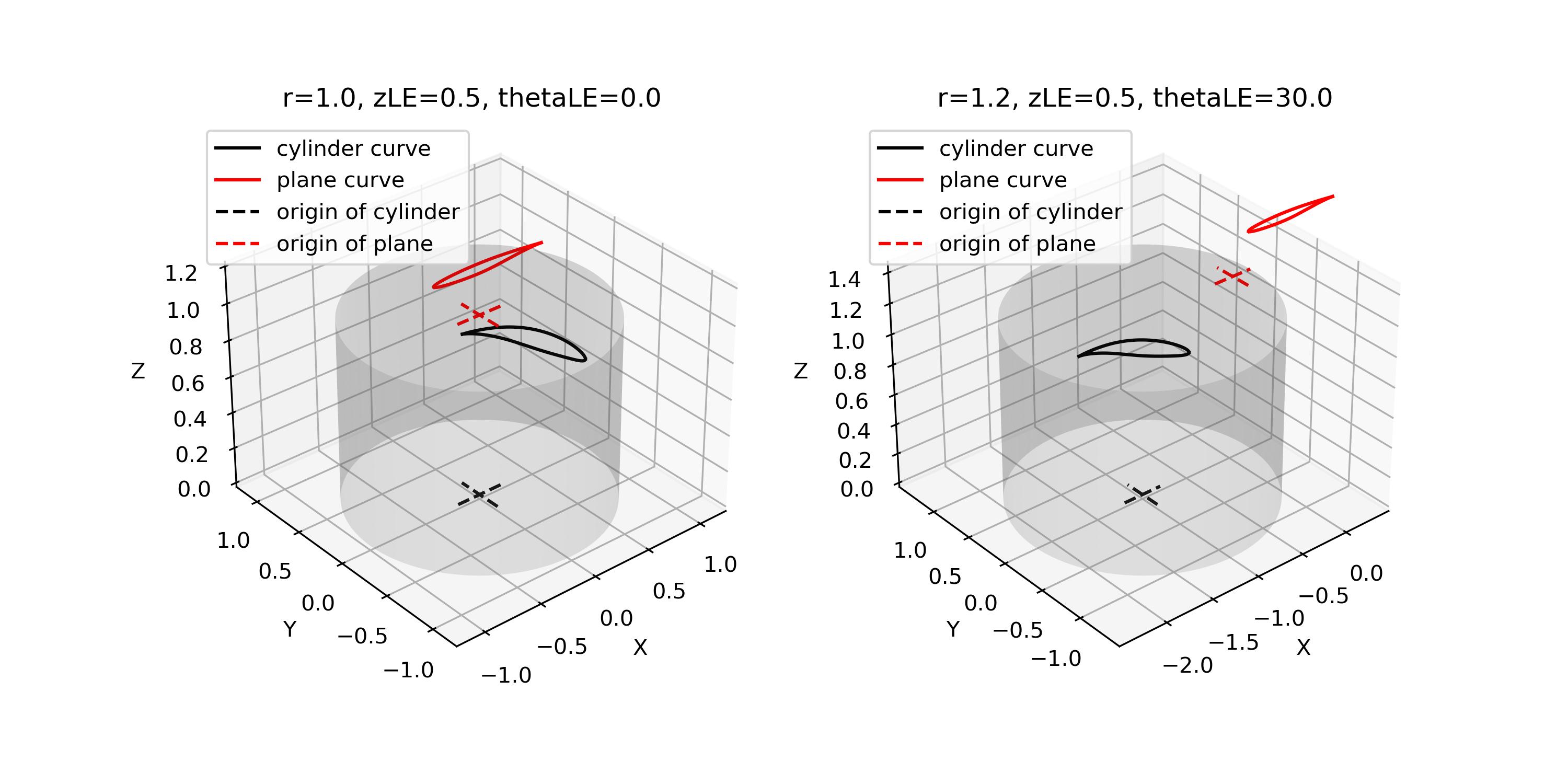
Figure 2.3.4 Cylinder to plane