2.1. 2D curve generation
2.1.1. CST base function
Figure 2.1.1 shows the base functions of the 6-th order CST method. The influence of parameter xn1 and xn2 is shown in the two sub-figures.
1x, y = cst_curve(101, cst, xn1=0.5, xn2=1.0)
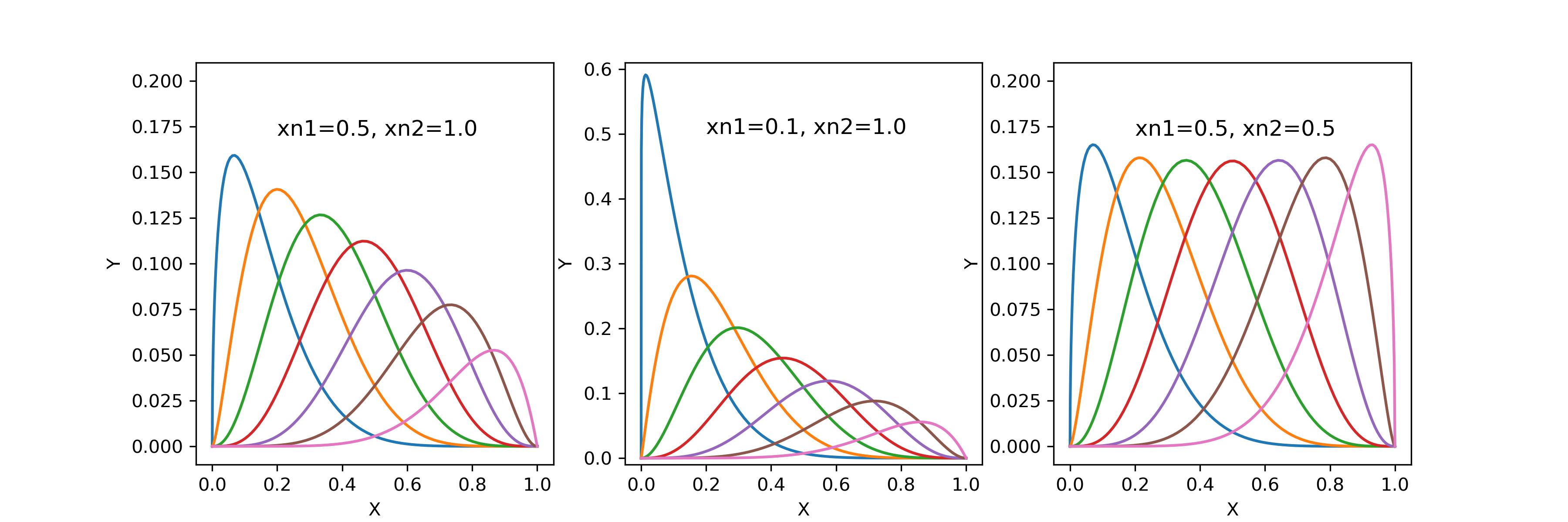
Figure 2.1.1 CST base function
2.1.2. Cosine distribution (X axis)
Figure 2.1.2 shows the density of a cosine distribution. The solid line is the gaussian density estimation of the point distribution. The stars show the actual points. The three different colors show the influence of the control parameter a0, a1, and beta.
1xx = dist_clustcos(101, a0=0.0079, a1=0.96, beta=1.0)

Figure 2.1.2 Cosine distribution
2.1.3. CST airfoil
Figure 2.1.3 shows the airfoil generated by CST method. The four airfoils have the same CST coefficients, but their t and tail settings are different.
The black airfoil is the original geometry defined by the cst_u and cst_l.
The red airfoil adds a finite tail thickness to the original geometry.
The blue airfoil applies a specified relative maximum thickness t to the original geometry.
The green airfoil adds a finite tail thickness to an airfoil, of which the t is specified.
1x, yu, yl, tmax, rLE = cst_foil(1001, cst_u, cst_l, x=None, t=None, tail=0.0)   # black
2x, yu, yl, tmax, rLE = cst_foil(1001, cst_u, cst_l, x=None, t=None, tail=0.02)  # red
3x, yu, yl, tmax, rLE = cst_foil(1001, cst_u, cst_l, x=None, t=0.05, tail=0.0)   # blue
4x, yu, yl, tmax, rLE = cst_foil(1001, cst_u, cst_l, x=None, t=0.05, tail=0.01)  # green
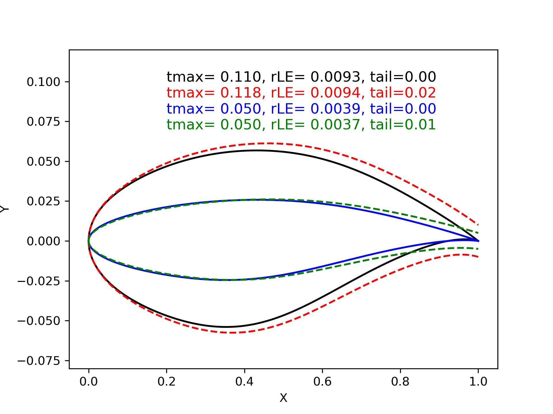
Figure 2.1.3 CST airfoil (changing t and tail)
Figure 2.1.4 shows the difference between airfoils when the CST parameter xn1 and xn2 are changed. The four airfoils have the same CST coefficients, the maximum relative thickness t is also fixed.
A smaller xn1 or xn2 gives the CST method more power to describe the shape in the leading edge or trailing edge. Sometimes, using a small xn1 is suggested when the leading edge needs delicate modification.
1x, yu, yl, tmax, rLE = cst_foil(1001, cst_u, cst_l, t=0.11)                   # black
2x, yu, yl, tmax, rLE = cst_foil(1001, cst_u, cst_l, t=0.11, xn1=0.1, xn2=1.0) # red
3x, yu, yl, tmax, rLE = cst_foil(1001, cst_u, cst_l, t=0.11, xn1=0.5, xn2=0.5) # green

Figure 2.1.4 CST airfoil (changing xn1 and xn2)
2.1.4. Fitting airfoil
Given an airfoil, you can use CST method for fitting.
1cst_u, cst_l = cst_foil_fit(x, yu, x, yl, n_cst=10, xn1=0.3, xn2=1.0)

Figure 2.1.5 Fitting airfoil with CST
2.1.5. Fitting blade
Given a blade (round tips at both ends), you can use CST method for fitting. The CST parameters xn1, xn2 need to be adjusted.

Figure 2.1.6 Fitting blade
1cst_u, cst_l = cst_foil_fit(xx, yu, xx, yl, n_cst=7, xn1=0.1, xn2=0.1)
2.1.6. Fitting curve
Given a curve, you can use CST method for fitting. The curve can be a unit chord length curve, i.e., x in [0,1]. It can also have any end point, but it must be a function after being transformed back to a unit curve, i.e., y=f(x).
1coef = fit_curve(x, y, n_cst=10, xn1=0.5, xn2=1.0)
2
3coef, scale, rotation, thick = fit_curve_with_twist(x, y, n_cst=10, xn1=0.5, xn2=1.0)
4
5coef = fit_curve_partial(x, y, ip0=200, ip1=501, ic0=2, ic1=11, n_cst=20, xn1=0.3, xn2=1.0)

Figure 2.1.7 Fitting curve with CST
You can also use CST to fit part of a curve. Sometimes this can be useful.

Figure 2.1.8 Fitting partial curve with CST
2.1.7. Curve curvature
Calculating the curvature of a curve is very useful in aerodynamic design.
1curvature = curve_curvature(x, y)

Figure 2.1.9 Curve curvature